Vectors are objects which can be scaled by real multiplication numbers and can be added.
Sequences, functions, and even objects that operate on functions can be vectors, leading a rich general theory of vectors.
Since this is an introductory course, we will largely constrain our study of vectors to those which lie in \(\R^n.\)
Definition2.1.1.
Let \(X\) and \(Y\) be two objects of whatever kind you like and let \(a\) and \(b\) be numbers. The expression \(aX+bY\) is called a linear combination of \(X\) and \(Y\) with coefficients \(\,a\) and \(b.\)
Definition2.1.2.
Vectors are objects which can form linear combinations.
In mathematics, linear combinations are of considerable importance. We may take linear conbinations of integers, of functions, and in this course we will take linear combinations of the fundamental objects on which we focus, ordered collections of real numbers, as defined in this Chapter.
In this course we build our intuition about general vectors, which we will encounter in Chapter 5, by first considering concrete vectors which are ordered lists of real numbers. To build such objects, we recall that an ordered pair in \(\R^2\) may be expressed as \((x_1,x_2).\) Generalizing this notion, we have the following.
Definition2.1.3.Points in \(\boldsymbol{\R^n}\).
Let \(n\in\N.\) The set of ordered \(n\)-tuples of real numbers is denoted \(\R^n.\) We denote points in \(\R^n\) as
where the individual \(x_i\)’s are elements of \(\R\) and are called coordinates.
Definition2.1.4.The origin in \(\boldsymbol{\R^n}\).
In \(\R^n\) the origin is the point
\begin{equation*}
(0,0,\ldots,0)
\end{equation*}
and may be denoted by \(O.\)
Remark2.1.5.
In this introductory section we use the letters \(P,Q,R\) to denote general points in \(\R^n.\) For \(P,Q\in\R^n\) the directed line segment from \(P\) to \(Q\) is denoted \(\vec{PQ},\) and the (degenerate) directed line segment from \(O\) to itself is denoted \(\vec{0}_n\) (or just \(\vec{0}\) if \(n\) is clear from the context).
Figure2.1.6.\(\vec{PQ}\) is the directed line segment from \(P\) to \(Q\)
Remark2.1.7.
For points \(P=(x_1,\ldots,x_n),\,Q=(y_1,\ldots y_n)\in\R^n\) we represent \(\overset{\rightharpoonup}{\boldsymbol{P}\boldsymbol{Q}}\) by the individual coordinate distances from \(P\) to \(Q,\) using the following notation:
Remark2.1.8.Each vector in \(\R^n\) is equivalent to many directed line segments.
It’s worth noting that, for example, the vector representation of the directed line segment from \(Q_1:=(3,-1,4)\) to \(R_1:=(-5,2,8)\) has precisely the same components as the vector representation of the directed line segment from \(O\) to \(P_1:=(-8,3,4)\text{;}\) the two directed line segments in \(\R^3\) differ only in their initial and terminal points. In fact, Remark 2.1.7 shows that a given vector can arise from any of an infinite number of directed line segments in \(\R^n,\) each of which have initial and terminal points whose components differ in exactly the same way.
There is a natural pairing between line segments from the origin to points \(P,\) and line segments from another fixed point \(Q\) to points \(R\) where the coordinates of\(P\) are the corresponding components of\(\overset{\rightharpoonup}{\boldsymbol{Q}\boldsymbol{R}}.\) This means that because we chose to represent directed line segments as in Remark 2.1.7 there is no substantive difference between a directed line segment \(\overset{\rightharpoonup}{\boldsymbol{O}\boldsymbol{P}}\) and any directed line segment \(\overset{\rightharpoonup}{\boldsymbol{Q}\boldsymbol{R}}\) with the same components, and we may freely substitute between such representations when convenient.
This is a necessarily long-winded way of noting that a vector actually represents an equivalence class of directed line segments where \(\overset{\rightharpoonup}{\boldsymbol{P}\boldsymbol{Q}}\equiv\overset{\rightharpoonup}{\boldsymbol{R}\boldsymbol{S}}\) if the corresponding components of each are equal. Another way of thinking of this is that 1) each such equivalence class is defined by a given length and direction and 2) any directed line segment in the equivalence class may be replaced by any other directed linne segment in the equivalence class. (The directed line segment from \(O\) to \(O\) may not be replaced by any other directed line segment.)
Figure2.1.9.Members of the same equivalence class of vectors \(\vec{v}\) of a given length and direction
Remark2.1.10.Pairing elements of \(\boldsymbol{\R^n}\) with vectors from the origin to points in \(\boldsymbol{\R^n}\).
Geometrically, there is another natural pairing which is useful to us, that between the set of points \(P\) in \(\R^n\) and the set of directed line segments \(\overset{\rightharpoonup}{\boldsymbol{O}\boldsymbol{P}}\) from the origin to \(P.\)
That is, for each point \(P\) in \(\R^n\) there exists a unique directed line segment starting at the origin and terminating at \(P,\) and for each directed line segment starting at the origin in \(\R^n\) there exists a unique terminal point \(P.\)
For this reason we may consider the elements of \(\R^n\) to be the set of such directed line segments. This is the content of the Definition 2.1.12 below.
Figure2.1.11.Each point \(P\) in \(\R^n\) corresponds to a directed line segment \(\vec{OP}\) from the origin to \(P\)
Definition2.1.12.Column vectors and row vectors.
Elements of \(\R^n\) represented as directed line segments from the origin to the point \((x_1,x_2,\ldots,x_n)\) in \(\R^n\) are called vectors (or \(n\)-vectors) and may be expressed as column vectors
In either representation the \(v_i\)’s and \(w_i\)’s are real numbers, called the components of \(\v\) and \(\w,\) respectively.
We call \(\v\) and \(\w\) vectors in \(\R^n.\)
Column vectors and row vectors are essentially the same types of objects, but their distinct arrangements are required for the upcoming topic of matrix-vector multiplication.
We will typically illustrate the algebraic properties of vectors in \(\R^n\) by using column vectors, but keep in mind that the same algebraic properties apply to row vectors as well.
We will occasionally encounter lists of vectors which we will write as \(\boldsymbol{v_1},\boldsymbol{v_2},\ldots,\boldsymbol{v_k}.\) This notation is not to be confused with the components \(v_i\) of a single vector \(\v.\) We will avoid situations in which we need to consider the components of a vector \(\boldsymbol{v_i}\) in a list of vectors wherever possible.
Definition2.1.13.The zero vector.
The zero vector \(\vec{0}\) is the unique vector with all components equal to \(0.\) When necessary we will indicate the size of the zero vector, as in
where it is understood that the latter zero vector has \(n\) components.
Definition2.1.14.Scalars.
A scalar is simply a real number, so called because of the context in which the scalar “scales” some vector by multiplication, as in Definition 2.1.15.
Definition2.1.15.Linear combinations in \(\R^n\text{:}\) vector addition and scalar multiplication.
Fix \(\u,\v\in\R^n,\,a,b\in\R.\) We define vector addition componentwise by
of \(\u\) and \(\v\) in which the scalars \(a\) and \(b\) are called the coefficients of the vectors \(\u\) and \(\v.\) (Compare with Definition 2.1.1.)
Linear combinations may be constructed from three, four, or as (finitely) many vectors as we wish.
The geometry of vector addition and subtraction. Our definition of vector addition aligns with the geometric interpretation of vector addition by placing them head to tail where their sum is the directed line segment from the tail of the first to the head of the second.
Figure2.1.16.Vector addition: \(\u+\v\)
We define vector subtraction \(\u-\v\) as the addition of \(-\v:\)
One particular linear combination of vectors is distinguished from all others. For any given set \(\left\{\vec{v_1},\vec{v_2},\ldots,\vec{v_k}\right\}\) of vectors, the zero vector \(\vec{0}\) is the linear combination of the vectors \(\vec{v_1},\vec{v_2},\ldots,\vec{v_k},\) with all coefficients equal to \(0.\) Such a representation of \(\vec{0}\) is called the trivial linear combination.
Definition2.1.19.CLC.
If \(\u,\v\in\R^n\) and \(a,b\in\R,\) we necessarily have that \(a\u+b\v\in\R^n.\) This property of \(\R^n\) is called closure under the taking of linear combinations, or CLC. We will discuss CLC in detail in Chapter 5.
Definition2.1.20.The vector norm.
Let \(\v\in\R^n.\) Then the Euclidean length or norm\(\,\|\v\|\) of \(\v\) is
In \(\R^2,\,\R^3\) we write \(\boldsymbol{\wh{e_1\!}}=\unit{\imath},\,\boldsymbol{\wh{e_2\!}}=\unit{\jmath}\) and in \(\R^3\) we also write \(\boldsymbol{\wh{e_3\!}}=\unit{k}.\)
Theorem2.1.25.
Every vector \(\v\in\R^n\) can be written as a unique linear combination of the canonical unit vectors in \(\R^n.\)
Proof.
The proof is left an as exercise.
Theorem2.1.26.Constructing unit vectors.
For any \(\v\in\R^n\setminus\left\{\vec{0}\right\},\) the vector \(\displaystyle{\frac{\v}{\|\v\|}}\) is a unit vector.
Proof.
The proof is left an as exercise.
Definition2.1.27.Normalization.
We normalize a nonzero vector when we divide by its length. The normalization of a nonzero vector \(\v\) is \(\displaystyle{\frac{\v}{\|\v\|}}.\)
Definition2.1.28.Parallelity and antiparallelity.
Two vectors \(\u,\v\in\R^n\setminus\left\{\vec{0}\right\}\) are parallel (antiparallel) if there exists a positive (negative) scalar \(k\) for which \(\v=k\u.\)
We denote the parallelity of \(\u,\v\) by \(\u\parallel\v\) and the antiparallelity of \(\u\,\v\) by \(\u\upharpoonleft\!\downharpoonright\v.\)
Parallel vectors point in the same direction while antiparallel vectors point in opposite directions.
Note that \(\vec{0}\) is not parallel nor antiparallel to any vector in \(\R^n.\)
Because of the ubiquitous use of \(x,y\) and \(x,y,z\) to represent coordinates in \(\R^2\) and \(\R^3\) respectively, we may occasionally use \(\begin{pmatrix}x\\y \end{pmatrix}\) or \(\begin{pmatrix}x\\y\\z \end{pmatrix}\) when considering vectors in \(\R^2\) or \(\R^3\) rather than using the subscript notation in (2.1.2) and (2.1.3).
Remark2.1.29.Components and coordinates.
Consider the point \((3,4)\in\R^2\) and its corresponding vector
In the context of locating a given point in the plane, the coefficients in the linear combination above are also called coordinates since their role in the expression \(3\begin{pmatrix}1\\0\end{pmatrix}+4\begin{pmatrix}0\\1\end{pmatrix}\) is to make explicit how far to proceed in each of the \(\begin{pmatrix}1\\0\end{pmatrix}\) and \(\begin{pmatrix}0\\1\end{pmatrix}\) directions, consistent with our intuitive notion of how to find the point \((3,4)\) in the plane.
But to find \((3,4)\) in the plane going \(3\) units in the \(x-\)direction and \(4\) units in the \(y-\)direction is not the only path. We could equally well go \(\frac{7}{2}\) units in the \(\left(\begin{array}{c}1\\1\end{array}\right)\) direction and \(\frac{7}{2}\) units in the \(\left(\begin{array}{r}-1\\1\end{array}\right)\) direction since
This notion holds for any point in the plane; we explore it a bit more in the next remark.
Remark2.1.30.Coordinatizing the plane.
Suppose \(\u,\v\in\R^2\setminus\left\{\vec{0}\right\}\) and that \(\v\) is not a multiple of \(\u.\)
The geometric interpretation of the set of all linear combinations \(a\u+b\v\) of two vectors \(\u,\v\) is essentially a change of coordinates
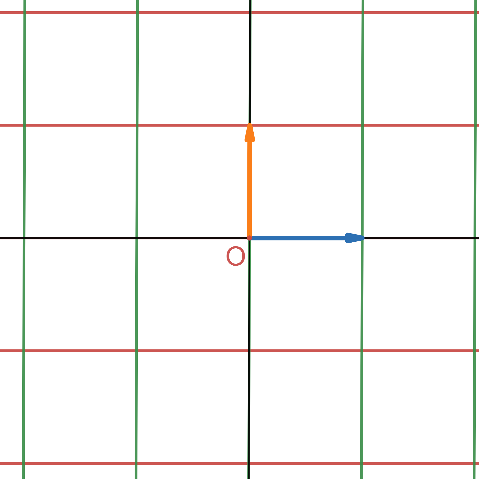
from the usual coordinatization of the plane with two orthogonal axes measured in increments of \(1\) unit:
Figure2.1.31.\(\R^2\) coordinatized by linear combinations of \(\left(\begin{array}{c}1\\0\end{array}\right)\) and \(\left(\begin{array}{c}0\\1\end{array}\right)\)
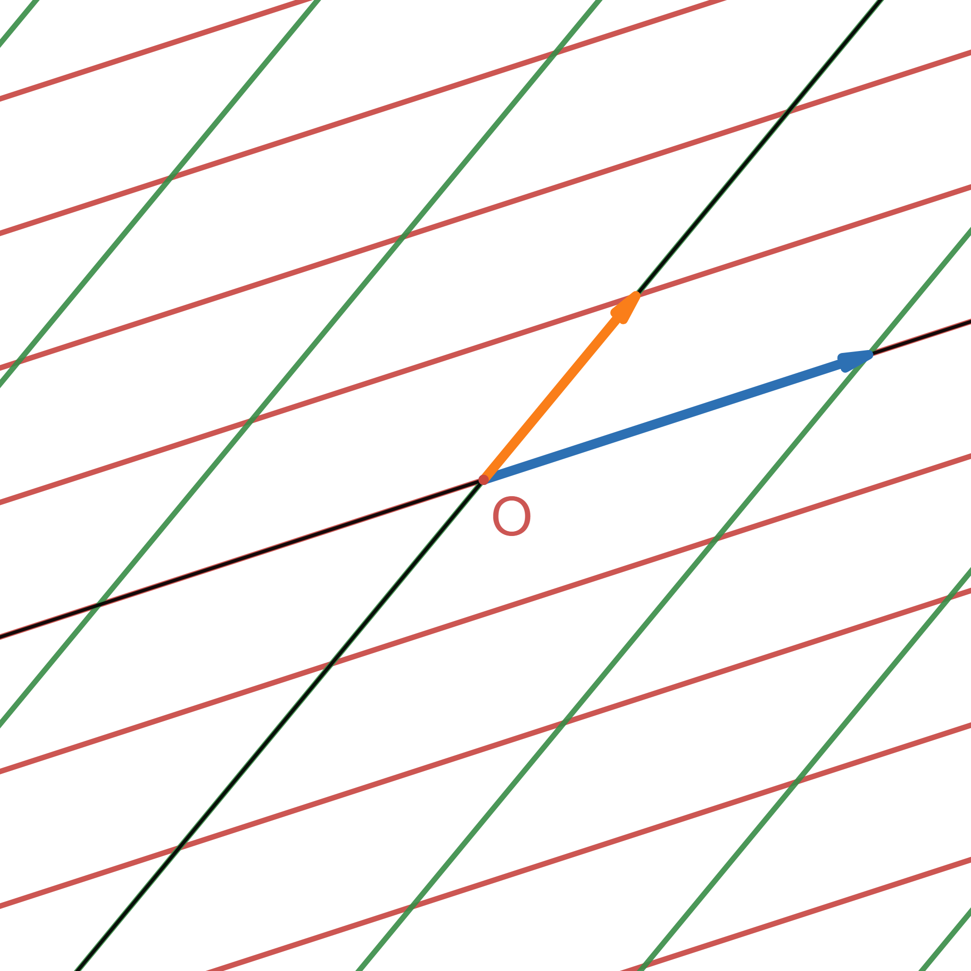
to the coordinatization of the plane having one coordinate axis along the direction specified by \(\u\) and measured in units of the length of \(\u,\) and the other coordinate axis along the direction specified by \(\v\) and measured in units of the length of \(\v\text{:}\)
Figure2.1.32.\(\R^2\) coordinatized by linear combinations of generic \(\u,\,\v.\) Resist the temptation to view this as a tilted plane; it’s a plane in the page coordinatized by a pair of typical vectors.
Indeed, consider the vector \(\left(\begin{array}{r}4\\-5\end{array}\right).\) In the usual coordinatization of \(\R^2,\) we have
so the coordinates are \((4,-5).\) But if for example \(\R^2\) is coordinatized by \(\left(\begin{array}{r}5\\2\end{array}\right)\) and \(\left(\begin{array}{r}2\\3\end{array}\right)\) we have
so the coordinates are \((2,-3).\) We can argue rigorously that the vectors \(\left(\begin{array}{r}5\\2\end{array}\right),\left(\begin{array}{r}2\\3\end{array}\right)\) can be used to coordinatize the plane, by fixing an arbitrary vector \(\left(\begin{array}{c}x\\y\end{array}\right)\in\R^2,\) assuming that some linear combination \(a\left(\begin{array}{r}5\\2\end{array}\right)+b\left(\begin{array}{r}2\\3\end{array}\right)\) equals \(\left(\begin{array}{c}x\\y\end{array}\right)\) and finding the coefficients \(a,b:\)
It turns out that if \(\u,\v\in\R^2\) are not collinear, then we can reach all of \(\R^2\) with linear combinations of \(\u,\v.\)
If however, \(\u,\v\) are collinear then we will not be able to reach all points in \(\R^2\) with a linear combination of \(\u\) and \(\v.\) Such linear combinations will reside only on the line consisting of multiples of \(\u\) (or of \(\v\)). For example, we cannot find a linear combination of \(\left(\begin{array}{r}-2\\1\end{array}\right),\left(\begin{array}{r}4\\-2\end{array}\right)\) which equals \(\left(\begin{array}{c}3\\1\end{array}\right).\) Assuming such a linear combination exists and trying to solve for the coefficients yields
which yields the equations \(3=-2a+4b\) and \(1=a-2b.\) Solving the second equation for \(a,\) substituting the result into the first equation ad simplifying yields \(3=-2,\) which shows that our assumption of the existence of such a linear combination implies an absurdity and hence could not have been correct in the first place. Thus no linear combination of \(\left(\begin{array}{r}-2\\1\end{array}\right),\left(\begin{array}{r}4\\-2\end{array}\right)\) equals \(\left(\begin{array}{c}3\\1\end{array}\right).\) More generally,
Similarly, in \(\R^3\) if some \(\u,\v,\w\) lie in a single plane, all linear combinations of \(\u,\v,\w\) will lie in that same plane, and there will be many points in \(\R^3\) which are not reachable with linear combinations of \(\u,\v,\w.\) But if \(\u,\v,\w\) are not coplanar, then we can reach all of \(\R^3\) with linear combinations of \(\u,\v,\w.\)
This notion holds in the general \(\R^n\) and leads to fundamental linear algebraic considerations - the solution of linear systems and more - which are central to the study of linear algebra.