Before setting up a weighted gradebook, one must
make some determinations about assignments and grading. Among those
decisions are the following:
What assignments, homework, tests, projects
will be included in the gradebook
What weight or percentage of the total
final grade will each assignment or entry be given; for example,
if the final test will be worth 25% of the total course grade, the
weight would be 25
What is the maximum points that will be
given to each assignment; for example the final will be graded on
the basis of 100 points, hence the maximum is 100, whereas the book
review may be graded on the basis of 20, so the maximum would be
20
What is the range for each letter grade;
for example 90-100 is an "A", 80-89 is an "B", etc.
Let's consider the following model. The
gradebook will include grades for the final test, a book review, three
assignments and participation in ten class periods.
The final will be worth 25%, the book
review 20%, each assignment 15% and each day of participation 1% for
a total of 100%. (This must add to 100%.)
The final test will be graded on a maximum
of 100 points, the book review and each assignments can receive up to
20 points and the daily will be graded on the basis of 2 points (good
participation, some participation and poor participation).
We'll let 90's be "A", 80's "B", 70's
"C", 60's "D" and below 60's "F".
Inital Setup
Setup columns
Blank
Last name of the student
First name
Assigned student number, i.e. the last four digits
of the V-number at WOU
Letter grade
Total class score
Book review weighted score
Assignment one weighted score
Assignment two weighted score
Assignment three weighted score
Final test weighted score
Total participation weighted score
Blank
Actual book review score
Actual assignment one score
Actual assignment two score
Actual assignment three score
Actual final test score
-28. Daily participation actual scores
Setup rows
Blank
Headings or titles of each column
The maximum possible points for each assignment
The weight of each assignment
A sample "ideal student" (for testing the computations)
A row for each student
A blank row after all the students
A row for counting the assignments
A row for averaging grades
General Setup
I typically color the borders and blanks
rows and columns a different color so I can quickly focus in on the
grades. I also color the second through five rows another color for
the same reason as well as columns that I want to "jump" out at me for
quick reference.
Entering Titles, Basic Values and Students'
Names
Enter students' names and numbers as appropriate
in columns B-D in rows 6 through whatever (for this assignment enter
about ten fictitious names).
Enter the appropriate headings or titles for each
column in row 2.
Enter the maximum possible points for each assignment
in row 3 and the weights in row 4
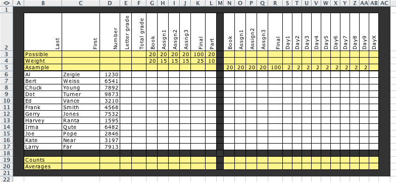
Name the sample student Asample and enter perfect
scores for this student in columns N through AB.
Select (highlight) cells and use Format/Cells to
add color and align text. Highlight a column (by clicking on the
letter at the top of the column) and use Format / Columns to change
its width.
Your project may look something like this:
Entering Formulas
Now we will be thinking a bit of math and a bit
of logic.
In cell G5 (that's the first weighted score for
our sample student, if you choose a different layout and don't end
up in G5), enter the formula =N5/G$3*G$4 . What is happening
is you're dividing the student's score (in cell N5) by the maximum
possible score (in cell G3) giving you the percentage score for
that student's assignment and then multiplying it by the weight
given to that assignment (which is in cell G4). Why the dollar
signs? In a moment we are going to quickly and easier replicate
that formula to all students and while the N5 will reflect the particular
student's score by changing to N6, and N7, and so on, the G3 and
G4 cell must remain absolute. The dollar sign does that.
After pressing Return or Enter, click on that same
cell again. Notice as you drag your cursor to different parts of
the cell, three different cursors appear. The hand will allow to
drag the contents of that cell somewhere else. Don't do that. The
big plus is the primary cursor, but the third (its shape varies
from computer to computer) appears when you near the lower right
corner of the cell. When it appears, click and drag to the
right over the cells for the three Assignments and the Final. Release
the mouse. Notice that the same formula is now in all the cells.
In the Participation cell, which we just ignored,
type =sum(S5:AB5)/L$3*L$4 and press Enter or Return.
In cell F5 type =sum(G5:L5) and press Return/Enter.
This should be 100.
In cell F4 type =sum(G4:L4) and press Return/Enter.
You could highlight F5 and copy and paste it into F4. This should
also be 100.
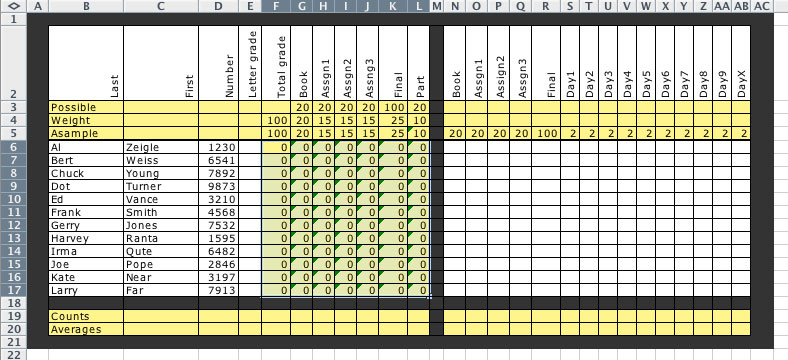
Click and drag your cursor across F5 to L5. Release.
Move to the special cursor in the lower right corner of L5. Click
and drag that cursor down over all the rows of students. Release.
Now the formulas are in all the cells.
Before we do the hard part, you should be seeing something like this.
That dragging may have messed up some formatting so you have to clean
that up.
Entering
More Formulas
This is more logic. We're going to use the statement "if the grade is
less than 90, the grade is not an 'A', but it that's not true it will
be an 'A'. In the spreadsheet cell E5, we will write =IF(F5<90,"not
A","A"). But we're going to compound that by putting this formula inside
of itself replacing the "not A" to recognize other letter grades. Trust
me on this one.
In
cell E5 (that's just to the left of the F4 where we put the total
class score several steps earlier), enter the formula =IF(F5<90,IF(F5<80,IF(F5<70,IF(F5<60,"F","D"),"C"),"B"),"A")
. Click and drag this cell to replicate this formula for all the
students.
Highlight
the cell in the Counts row in the First Name column. The top menu
bar, select Insert and then Function. When the new little window
appears, select All in the left column and COUNTA in the
right column. When the next window appears, click on the little
triangle to the right of the first textbox; and then highlight all
the first names. Click on that same little triangle and click OK.
Repeat
the above process in the Counts row in the columns where you will
be entering the scores using the COUNT function. COUNTA counts
words, COUNT counts numbers.
Repeat
the above process in the Averages row in the appropriate columns
using the AVERAGE function. Until you enter scores this may
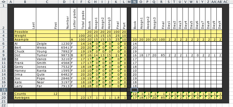
look crazy.
The sample below includes some scores for one completed assignment and
all scores for one student so one might see how this works.
Putting
in on the Web
To share this information with the students and parents, you may put
this on the Internet, obviously without names. Use only their numbers.
Highlight
the entire rows of all the students by clicking on the number
in front of the first row with student information and dragging
down to the last row with student information. In this sample that
would be 6-17. Be certain that the entire row is highlighted and
not just a couple columns.
Select
Data, then Sort from the menu bar. Sort on the column with
the students' numbers (probably column D).
Highlight
all the students' scores including the headings but certainly
not the names. In this example that would be from cell D2 to AB17.
Notice that counts and averages were not selected as you may not
want to share that information.
Select
File and then Save as Web Page in the menu bar. Save in your
public_html folder and give it an appropriate name making certain
that the .htm or .html is on the end of the name.
Check
your work online by going to your webpages at www.wou.edu/~username.
Office hours: Tuesday mornings: 9:00 - noon
Thursday mornings: 9:00 - noon
Other times aby appointment
Also contact me through email at saxowsd@wou.edu
or denvygail@saxowsky.com