Formatting The Appearance of a Workbook
You will learn how to format an
Excel workbook in this part of the tutorial.
 Open your "checks" workbook if it isn't
already opened.
 Select the first row of the "checks" workbook,
by clicking in the cell containing the bold face 1.
Observe:

You have just selected what Excel describes as a
range.
The Concept of a Range
A range is a rectangular block of cells. Many things
are accomplished in Excel using ranges. For instance,
the format used to display values can be changed for
an entire range. All the values in a range can be
referred to when writing a formula. A range of cells
can also be protected, which means the contents of the
cells cannot be altered. Ranges can also be named.
Excel also allows you to select discontinuous
ranges. You will learn how to do this further on in the
tutorial.
 With the range of cells A1:F1 selected, click on the Bold
button and Center alignment button.
This formatting should have made the text too big
for the cells.
 Adjust the column widths of the columns.
Your workbook should look similar to the following:

Selecting Discontinuous Ranges
 Select the first range of cells: A3:A6.
 Hold down the Ctrl key and select
the range of cells: C2:C6.
Observe:

 Click on the Center alignment button.
Let's format the dates.
Formatting Dates and Numbers
The basic formatting rule "select and then do"
is used when working with Excel.
 Select the range of cells: B3:B6.
 Choose Cells from the Format menu.
The following Format Cells dialog box should
appear:
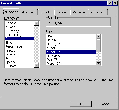
 Click on the Number tag if it is not already
displayed.
 Within the Category box highlight Date to view
all the Format Codes.
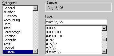
 Scroll through the options in the Format Codes.There
is no format that displays as: Aug. 8, 96. You can custom
format by typing in the Code box.
 Within the Code box, type in the following custom
format:
 Click on the Center alignment button to align
the dates.
Now let's format the dollar amounts.
 Select the discontinuous range displayed below:

Remember to select the first region, then hold down
the apple key when you select the remaining regions.
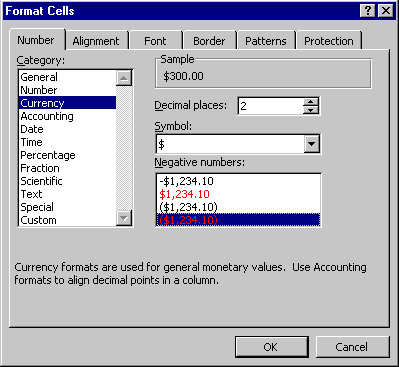
 Choose Cells from the Format menu.
 Click on the Number tab if it is not already
displayed.
 Within the Category box highlight Currency.
 Select the following Format Code and then click OK:
 Click on the Center alignment button to
align the dollar amounts.
Note that you could have selected the whole
"checks" workbook and then clicked on the
Center button.
Your "checks" workbook should look as follows:

Let's insert a row between
row 2 and row 3 in the "checks" workbook, to
make the workbook more appealing to the eye.
 Select row 3 by clicking on the bold face 3.
 Choose Rows from the Insert menu.
You have now learned how to format an Excel document.
Note that within the Format Cells dialog box you
can format the borders of the cells, change the
color,pattern, and shading of the cells and
protection of cells can be set there too.
You have completed your first workbook. It is time
to preview it.
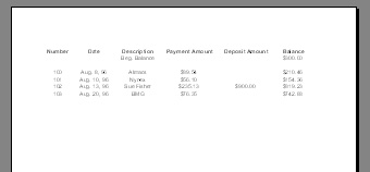
Choose Print Preview from the File
menu.
Observe:
 Click on the Close button to
return you to the workbook.
Observe the dotted line between column E and
column F, the dotted line indicates that there
will be a page break there.
What you want to do is actually flip the table
so it will fit on the whole page. You can do
this by choosing Page SetUp from the
File menu.
 Choose Page SetUp from the
File menu.
The following Page Setup dialog should
appear:
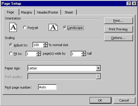
 Click on the Page tab if it isn't already
displayed.
 Within the Orientation box click on Landscape
and then click on the OK button.
Observe the dotted line (indicating a page break)
at the bottom of your workbook and running horizontal.
 Preview your "checks" workbook and then print
a copy of it.
 When your done printing close the "checks" workbook.
You are now ready to learn some advanced features of
Excel 5.0.
 Open your "checks" workbook if it isn't
already opened.
 Select the first row of the "checks" workbook,
by clicking in the cell containing the bold face 1.

 With the range of cells A1:F1 selected, click on the Bold
button and Center alignment button.
 Adjust the column widths of the columns.

 Select the first range of cells: A3:A6.
 Hold down the Ctrl key and select
the range of cells: C2:C6.

 Click on the Center alignment button.
 Select the range of cells: B3:B6.
 Choose Cells from the Format menu.

 Click on the Number tag if it is not already
displayed.
 Within the Category box highlight Date to view
all the Format Codes.
 Scroll through the options in the Format Codes.There
is no format that displays as: Aug. 8, 96. You can custom
format by typing in the Code box.
 Within the Code box, type in the following custom
format:

 Click on the Center alignment button to align
the dates.
 Select the discontinuous range displayed below:

 Choose Cells from the Format menu.
 Click on the Number tab if it is not already
displayed.
 Within the Category box highlight Currency.
 Select the following Format Code and then click OK:

 Click on the Center alignment button to
align the dollar amounts.

 Select row 3 by clicking on the bold face 3.
 Choose Rows from the Insert menu.

 Click on the Close button to
return you to the workbook.
 Choose Page SetUp from the
File menu.

 Click on the Page tab if it isn't already
displayed.
 Within the Orientation box click on Landscape
and then click on the OK button.
 Preview your "checks" workbook and then print
a copy of it.
 When your done printing close the "checks" workbook.