Advanced Excel (Copying Cells)
In this part of the tutorial you will be creating
a workbook and learning how to fill a cell or range
of cells with formulas to speed data entry.
 Find and Open Excel 97 if it isn't already open.
 Choose New from the File menu to
start a new workbook if there isn't a new workbook
open.
 Choose Formula Bar from the View menu
to display the formula bar.
You will be creating an income statement worksheet.
 Make the entries displayed below:
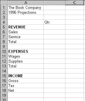
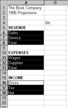
 Select the text below the bold faced headings,
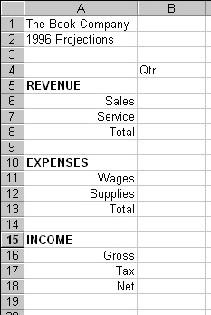
and right justify the text.
Remember to hold down the Ctrl key when selecting
a discontinuous range.
Observe:
Your workbook should look as follows:
Before you enter any formulas, let's name some of
the cells in your worksheet.
Naming Cells
Excel allows you to name any cell, range, or value
in a workbook. You can then use this name to refer to
the cell,range, or value. Names make formulas easier
to read, understand, and maintain. You can change or
delete names that have been defined previously. Names
appear in the reference area of the formula bar when
you select a named cell or range.
 Select cell B6 and choose Name from the
Insert menu, and choose Define from
the Name submenu.
 Within the Names dialog box, Excel provides
a possible name: Sales. This is fine. Click the
OK button.
 Select cell B7 and name it: Service.
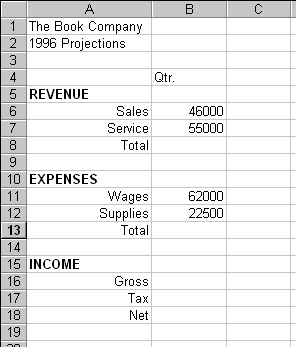
 Enter the following constants into your workbook:
 Select cell B8 and enter the formula that sums
Sales and Services.
 Save your workbook as "company".
The formula in cell B8 should be either the formula
=B6+B7 or =SUM(B6:B7). The formula is summing up the
two cells directly above cell B8. If you look at cell
B13, it will need a formula too. The formula in cell
B13 will also sum up the two cells directly above it.
This is where Excel's Copy command is useful.
What you can do is copy the formula from one cell
to another cell.
Copying From One Cell to Another Cell
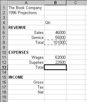
 Select cell B8.
 Choose Copy from the Edit menu.
Excel places a marquee around the cell.
 Select cell B13 and choose Paste from
the Edit menu.
Your company workbook should look as follows:
 Press the Escape key on your keyboard to cancel the
marquee.
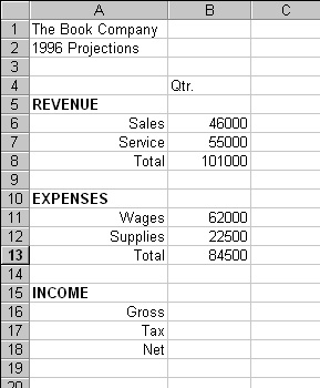
 Select cell B13. The formula should be =B11+B12 or
=SUM(B11:B12). That is the formula has summed the
two cells directly above cell B13.
Your company workbook should look as follows:
 Save your work before proceeding.
You now know how to copy a formula from one cell
to another. Next, in order to duplicate the Qtr.
heading across columns C through E, you will make
a copy from one cell to several other cells.
Copying From One Cell to Several Cells
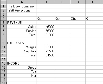
 Select cell B4 and choose Copy from the
Edit menu.
 Highlight the range C4:E4.
 Choose Paste from the Edit menu.
 Press the Escape key to remove the marquee.
Your company workbook should look as follows:
 Center the Qtr. headings.
 Save your work before proceeding.
The next step is to fill in the range C6:E7 with
projected revenues.
 Select cell C6 and enter the formula =B6*1.08.
 Choose Copy from the Edit menu.
 Highlight the range C6:E7.
Observe:
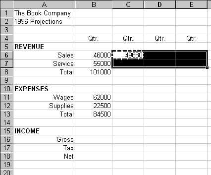
 Choose Paste from the Edit menu.
Your company workbook should look as follows:
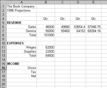
 Highlight the cells in the range C6:E7 and observe
the cell's formulas. In each cell the formula multiplies
the cell directly to the left of it by 1.08.
You can also copy data and formulas from one location
on the workbook to another using the Fill command.
 Find and Open Excel 97 if it isn't already open.
 Choose New from the File menu to
start a new workbook if there isn't a new workbook
open.
 Choose Formula Bar from the View menu
to display the formula bar.
 Make the entries displayed below:

 Select the text below the bold faced headings,
and right justify the text.


 Select cell B6 and choose Name from the
Insert menu, and choose Define from
the Name submenu.
 Within the Names dialog box, Excel provides
a possible name: Sales. This is fine. Click the
OK button.
 Select cell B7 and name it: Service.
 Enter the following constants into your workbook:

 Select cell B8 and enter the formula that sums
Sales and Services.
 Save your workbook as "company".
 Select cell B8.
 Choose Copy from the Edit menu.
 Select cell B13 and choose Paste from
the Edit menu.

 Press the Escape key on your keyboard to cancel the
marquee.
 Select cell B13. The formula should be =B11+B12 or
=SUM(B11:B12). That is the formula has summed the
two cells directly above cell B13.

 Save your work before proceeding.
 Select cell B4 and choose Copy from the
Edit menu.
 Highlight the range C4:E4.
 Choose Paste from the Edit menu.
 Press the Escape key to remove the marquee.

 Center the Qtr. headings.
 Save your work before proceeding.
 Select cell C6 and enter the formula =B6*1.08.
 Choose Copy from the Edit menu.
 Highlight the range C6:E7.

 Choose Paste from the Edit menu.

 Highlight the cells in the range C6:E7 and observe
the cell's formulas. In each cell the formula multiplies
the cell directly to the left of it by 1.08.