---

The Fill Command

---

Select the range B8:E8.

Choose Fill from the Edit menu, and from the Fill submenu choose Right.

Your company workbook should look as follows:


The projected expenses in the range C11:E12 are computed as 1.02 times the value of the previous quarter.

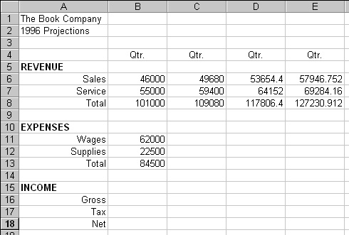
Select cell C11 and enter the formula =B11*1.02.

Select the range C11:C13 and choose Fill from the Edit menu, and from the Fill submenu choose Down.

Your company workbook should look as follows:


Excel provides another means of copying text, values, or formulas from one cell to other cells. Excel provides the AutoFill command. AutoFill copies cell's contents with out using the menu. You work directly on the workbook using the mouse.

---

Copying Cells Using AutoFill

---

The AutoFill feature is used to copy formatting, formulas, or all cell contents, or to perform different types of series extensions. For example, if you type Monday and Tuesday in consecutive columns, and then drag the fill handle to the right, Excel fills Wednesday, Thursday and so on into selected cells.

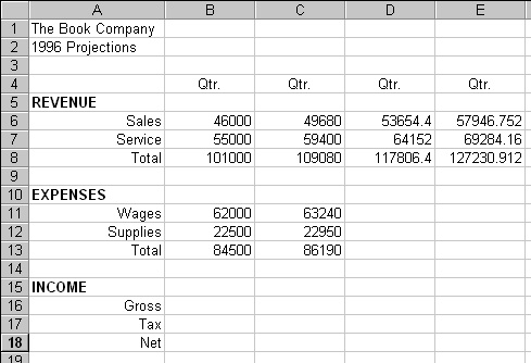
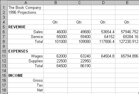
Select cell C11. Cell C11 contains the formula you want to copy.

Observe the fill handle located in the lower-right corner.

Place your mouse over the fill handle, until the arrow becomes a black cross.

Drag the fill handle across the cells D11 and E11 and then release the mouse button.

Your company workbook should look as follows:


You can also select more than one cell and then use the AutoFill command to copy.

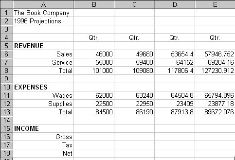
Select the range C12:C13.

Drag the fill handle across the range D12:E13.

Your company workbook should look as follows:


You have now learned how to copy in Excel. You may use any method above to finish the company workbook.

Select cell B16 and enter the formula =B8-B13.
(Gross Income is equal to Total Revenue minus Total Expenses)

Select cell B17 and enter the formula =B16*.22.
(The Tax is 22%)

Select cell B18 and enter the formula =B16-B17.
(Net Income is Gross Income minus the Tax)

Your company workbook should look as follows:


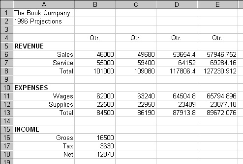
Copy the formulas in the range B16:B18 to the range C16:E18 using any method you would like.

Your company workbook should look as follows:


You have almost completed your company workbook. There is one more column to enter.

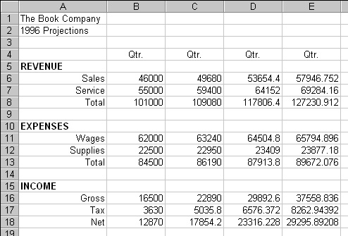
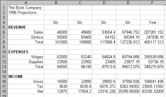
Select cell F4 and enter and center the text: Year.

Select cell F6 and enter the formula =SUM(B6:E6).

Copy the formula in cell F6 into the following ranges: F7:F8, F11:F13, and F16:F18.

Your completed company workbook should look as follows:


Save your changes.

Your company workbook is complete. You can now use the power of Excel's automatic recalculation feature. You can now use What If? analysis.

---

What If? Analysis

---

What If? analysis involves three steps:

1. First, you ask a What If? question about your workbook. For example, "What if the total revenue in the first quarter was $5000?"
   
   
2. Second, you alter the appropriate cell or cells in your workbook. In this case it would be cell B8.
   
   
3. Third, you observe how the different values in the workbook change.
   

Experiment with a What If? analysis and enter $5000 into cell B8.

Observe that the Income entries are now negative.

Undo the entering of $5000 or enter $101000 in cell B8.

Now that you are done with your company workbook, you can learn one more of Excel's advanced features: Linking.

Next Topic: Linking Documents

Main Menu